RNN and LSTM (Recap)

On output, one fashion is a single output $\boldsymbol{y} \in \mathbb R^{m}$ (at the final time step $T$), that is to say: $$ f(\{\boldsymbol{x}_{t}\}) = \boldsymbol{y} $$ This can be useful in sentiment analysis.

• This seems to be a problem even approachable by regression or classification.
• But notice that the input dimension can be large ($n\times T$), or even not fixed length (since $T$ is sample-dependent). Although truncation or padding can be applied, but still, it seems to be suboptimal to model like this.

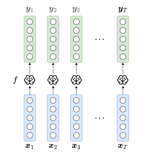
Another way to model this problem is that we seek a function that predicts a $\boldsymbol{y}_{t}$ for each $\boldsymbol{x}_{t}$, that is to say, $$ f(\boldsymbol{x}_{t}) = \boldsymbol{y}_t $$ and we only take the final outcome $\boldsymbol{y}_{T}$ as the targeted outcome. The progresses here are:

• Input dimension has been reduced (from $n \times T$ to $n$), which is not sample-dependent anymore!
• The downside for this formulation is that there is no memory of the previous information at all.
• Output at each step is also interesting in translation or language generation task, where we care about all the outputs $\{\boldsymbol{y}_{t}\}$.
• This is also related in return_sequence option in Keras.

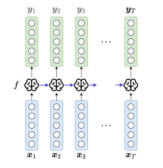
To add dependency, we can formulate the model as $$ f(\boldsymbol{x}_{t}, \boldsymbol{y}_{t-1}) = \boldsymbol{y}_{t}, \qquad t=1,2,\ldots, T. $$ with inital condition of $\boldsymbol{y}_{0}$ (set as $\boldsymbol{0}$ or something else).

• This formulation includes (immediate) short-term memory explicitly.
• The input dimension becomes $n + m$, slightly larger than Formulation 2.
• The output $\boldsymbol{y}_{t}$ is sometimes called hidden states (denoted as $\boldsymbol{h}_{t}$) in some context. Sometimes, there will be another $\tanh$ transformation applied, sometimes, it is just a copy of $\boldsymbol{h}_{t}$. It is especially so in the context of LSTM.
• However, RNN suffers from a problem called lack of long-term dependency (in practice, not theoretically). (Though "Why we need long term memory?" is still arguable.)
• The number of output is the same as the number of inputs, which is probably not flexible enough.

To really get one step closer to translation or conversational robots, seq2seq proposed by Mikolov is one milestone. Basically, it is a combination of formulation 1 (encoding — to understand the input) and 2 (decoding — to generate output).

• Cell state: $\mathbf c_{t}$. (a.k.a. carry state as commented in Keras source code.)

  • Why? keep "encoded" long-term memory.
  • Key point: only linear transformation applied to this cell.
  • Dimension: $\mathbb R^{n}$.

• Gates:

  • Including: forget gate ($\mathbf f_{t}$), input gate ($\mathbf i_{t}$), output gate ($\mathbf o_{t}$).
  • Dimension: $\mathbb R^{n}$.

Put in language:

1. Compute forget gate (to forget some past memory)
2. Compute input gate (to digest some new memory)
3. Compute output gate (be mindful on what to output)
4. Compute candidate memory
5. Update memory by
6. Compute output

Formula-form: $$ \begin{aligned} \mathbf{f}_{t} &= \sigma( \mathbf{W}_{\mathbf{f}} [\mathbf{h}_{t-1}, \boldsymbol{x}_{t}])\\ \mathbf{i}_{t} &= \sigma( \mathbf{W}_{\mathbf{i}} [\mathbf{h}_{t-1}, \boldsymbol{x}_{t}])\\ \mathbf{o}_{t} &= \sigma( \mathbf{W}_{\mathbf{i}} [\mathbf{h}_{t-1}, \boldsymbol{x}_{t}])\\ \widetilde{\mathbf{c}}_{t} &= \tanh(\mathbf{W}_{\mathbf{c}} [\mathbf{h}_{t-1}, \boldsymbol{x}_{t}])\\ \mathbf{c}_{t} &= \mathbf{f}_{t} \odot \mathbf{c}_{t-1} + \mathbf{i} \odot \widetilde{\mathbf{c}}_{t}\\ \mathbf h_{t} &= \mathbf{o}_{t} \odot \tanh(\mathbf{c}_{t}) \end{aligned} $$

1. Use ReLU
2. batch normalization
3. ResNet
4. weight initialization

1. Re-design your model using fewer layers
2. smaller batch size
3. truncated backprop through time
4. use LSTM
5. use gradient clipping
6. use weight regularization
7. batch normalization